Announcements
Integration Time Calculator (ITC)
In the four sections of this form, select the appropriate astronomical source, telescope and instrument configuration, observing conditions, and observation parameters. Click on the calculate button (![]() ) at the bottom of any section to submit the parameters from all the sections to the server or the reset button (
) at the bottom of any section to submit the parameters from all the sections to the server or the reset button (![]() ) to reset all parameters to their defaults. The results are reported in a separate web page that can be resized and printed.
) to reset all parameters to their defaults. The results are reported in a separate web page that can be resized and printed.
See the ITC Help for general guidance on use of the Integration Time Calculators, and the (more info) links for specific help on each section of the form.
If the form below does not appear then you may need to check with your system administrator about allowing communication with http://itc.gemini.edu:9080 through your firewall.
Exposure time limits
NIR background is highly variable
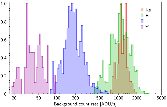
The NIR background is highly variable between nights, varying by factors 5-8 in Y, J and H, and factors 2-3 in Ks-band. Among other things this depends on the length of the observation, airmass, time after sunset (J-band), air and mirror temperature (Ks-band), solar flux during the day, precipitable water vapor, physical conditions in the high atmosphere, etc. Within a typical individual observing sequence variations are much smaller, changing perhaps by 10% (Y, Ks), 15-25% (J), and 20-30% (H). These are guidelines, only.
Once your program got accepted, the time allocation cannot be changed. Your observations are subject to the background levels encountered during the nights at which your target is observed. You may end up with better or worse S/N than requested. The following is therefore very important:
Always include a note in the Phase 2 Observing Tool, addressed to the observer, with an indication of what background levels your program can tolerate. The observer needs to know how to adjust integration times at the beginning, and then the sequence should ideally run without further modification. If exposure times were cut short, you can ask your contact scientists to add more steps to the sequence while staying within the allocated time.
Fig: Long-term (2012-2017) sky background rates observed with FLAMINGOS-2, normalized to same height for better comparison. Note that within a typical observing sequence variations are much smaller, on the order of 10-20%.
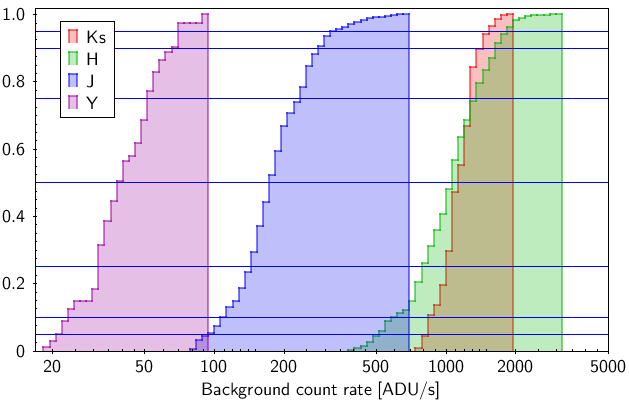
Fig: Same as above, but showing the cumulative histograms with the 5, 10, 25, 50, 75, 90 and 95 percentiles indicated by the horizontal lines. Using this plot you can evaluate the risk of exceeding a certain background level (or the chance to stay below).
The following table was built from the cumulative histograms shown above, listing the exposure times for which a background level of 10 kADU is exceeded with a certain probability. Example usage:
- With a 10s integration time in Ks you will get 10 kADU or more in 75% of the cases.
- Multiply the exposure times with factors 1.5 and 2, if you want to know the risk of exceeding 15 and 20 kADU, respectively.
- Say you have fairly bright targets, and want to stay below 13 kADU in K-band with 90% probability to allow for enough dynamic headroom. Take the 10% line (the complementary probability), which gives you 7s. Multiply by 1.3 to go from 10 kADU to 13 kADU, yielding 9 s integration time.
| Probability of exceeding 10 kADU |
Y texp [s] |
J texp [s] |
H texp [s] |
Ks texp [s] |
| 5% | 140 | 29 | 5 | 6 |
| 10% | 150 | 34 | 6 | 7 |
| 25% | 180 | 42 | 7 | 8 |
| 50% | 250 | 56 | 9 | 9 |
| 75% | 310 | 69 | 12 | 10 |
| 90% | 360 | 91 | 16 | 11 |
| 95% | 370 | 102 | 19 | 12 |
Phase 1+2: Planning exposure times
When planning your Phase 1+2 you face the following problem. You must balance desired S/N, remaining dynamic range above background, detector linearity and instrument overheads against each other, in the context of the long- and short-term background variations. The longer you expose, the higher the background level, and the less dynamic (and linear) range remains for your science targets. The less headroom you leave, the higher the risk that smaller short-term variations drive your background too high. On the contrary, the shorter your exposure times, the higher the fractional overhead (15 seconds for readout and data transfer). Note that FLAMINGOS-2 cannot do any on-detector arithmetics.
How should (or could) you go about this? Your mileage may vary.
First, assume median count rates of 50, 200, 1100, 1200 ADU/s for filters Y, J, H and Ks, respectively. These are rounded up a little from the median count rates, and also correspond to the most common background level encountered. Like this, you have equal chances of getting higher or lower S/N when the sequence is executed without modifications.
Second, use the ITC to find out how many total ADU/s you get in a single exposure for the source and the background. Note that in its current version (July 2017), the ITC assumes 64, 235, 2380, 730 ADU/s, respectively. It is too pessimistic in H, and a bit too optimistic in Ks (all for an airmass 1.5). You can then decide on the best integration time for your program, and the total time request.
Example:
You image distant galaxies in Ks-band, barely visible in single exposures. Then you can easily accept a background level of 20-25 kADU, and an integration time of 16 s would give you 19.2 kADU for the median count rate listed above. Once the sequence is started, the background will vary within perhaps 10% (see the paragraph at the very top). Even if the background rate was 1500 ADU/s (95 percentile) in that night at the start of the sequence, you'll be fine. If you require 2MASS sources in the field for calibration, shorter exposure times are indicated to keep the 2MASS sources within the linear range. Alternatively, maintain the long integration times and observe a photometric standard before the science sequence.
If you observe brighter sources, e.g. a star cluster in H-band, then you'll have to cut back on the individual integration times to accomodate the source, and the higher potential background fluctuations during the sequence (20-30%).
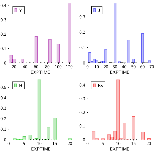
Fig: For reference, these are the individual exposure times chosen by our PIs for the data displayed in the histograms above.


